How We Found Our Stars
Table of Links
Abstract and 1 Introduction
-
Sample selection and properties
-
Results
-
Discussion
-
Concluding remarks and References
Appendix A: Sample selection
Appendix B: Properties of the TOIs in this work
Appendix C: Pre-MS estimates
Appendix A: Sample selection
The description of the TOIs catalog is in Guerrero et al. (2021), but the updated list including 6977 TOIs[2] was taken as a departure point for selecting the sample. The previous list was initially filtered by only considering the sources that according with the TOIs catalog have: i) A light curve that is compatible with planetary transits (i.e., not rejected as false positives, not related with instrumental noise, or not classified as eclipsing binaries, with sources showing centroid offsets also discarded, stellar variables, or ambiguous planet candidates). ii) An orbital period of P < 10 days. For the few exceptions where two or more planets are associated to a given star, only the one with the shortest period was considered.
\ The resulting list was cross-matched with the Gaia DR3 catalog of astrophysical parameters produced by the Apsis processing (Creevey et al. 2023; Fouesneau et al. 2023). A radius of 1" was used to cross-match the TOIs and Gaia coordinates. A second filter was then applied, keeping the single sources that have: iii) Gaia DR3 values for L∗, M∗, and R∗. iv) An evolutionary status consistent with being in the MS (i.e., Gaia DR3 "evolution stage" parameter of ≤ 420). After the previous process, the initial number of TOIs is reduced by more than a factor of 3. Among the resulting list, 25 intermediate-mass stars with light curves having either a "confirmed planet" (CP) or "Kepler planet" (KP) status in the TOIs catalog were identified. These are all TOIs with Gaia DR3 masses > 1.5M⊙ and confirmed short-period planets (i.e., less massive than 13 MJup) currently identified in the Encyclopaedia of Exoplanetary Systems[3]. This sample was kept and the remaining intermediate-mass stars were further filtered as follows.
\ 
\ In addition, we selected the 298 low-mass stars with CP or KP status in the TOIs catalog and inferred planetary sizes compatible with giant, gas made planets similar to those around the intermediate-mass sample. This list results from the step iv described above, constituting all TOIs with Gaia DR3 masses ≤ 1.5 M⊙ and confirmed short-period planets, in accordance with the Encyclopaedia of Exoplanetary Systems.
\
Appendix B: Properties of the TOIs in this work
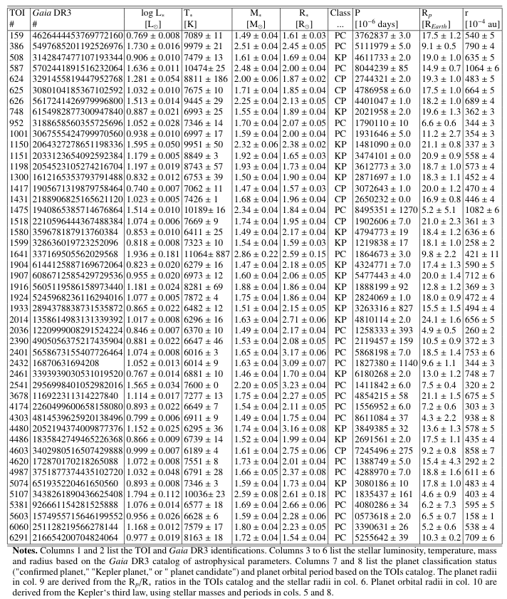
Table B.1 lists main parameters of the 47 TOIs with intermediate-mass stars analysed in this work. Values for the stellar luminosities, temperatures, masses and radii were taken from the Gaia DR3 catalog "I/355/paramp: 1D astrophysical parameters produced by the Apsis processing chain developed in Gaia DPAC CU8". Among the different estimates for the effective temperatures available in that catalog, we selected the ones derived from BP/RP spectra. The main reason for this selection is that such temperature estimates cover a larger sample of stars than the rest. In addition, we checked that relative errors are mostly < 10% when compared with effective temperatures derived from higher resolution spectra also available in that catalog. Errorbars for the stellar parameters refer to the lower (16%) and upper (84%) confidence levels listed in the Gaia DR3 catalog. The planet classification status come from the "EXOFOP disposition" column in the TOIs catalog, from which the orbital periods and errors were also taken. Planet radii were derived from the Rp/R∗ values in the TOIs catalog and the stellar radii in the Gaia DR3 catalog. The propagation of the corresponding uncertainties served to provide the final errorbars listed for the planet radii. Finally, orbital radii were derived from the Kepler’s third law assuming that the planet mass is negligible compared with the stellar mass. Errorbars come from the propagation of the uncertainties in the orbital periods from the TOIs catalog and in the stellar masses from the Gaia DR3 catalog.
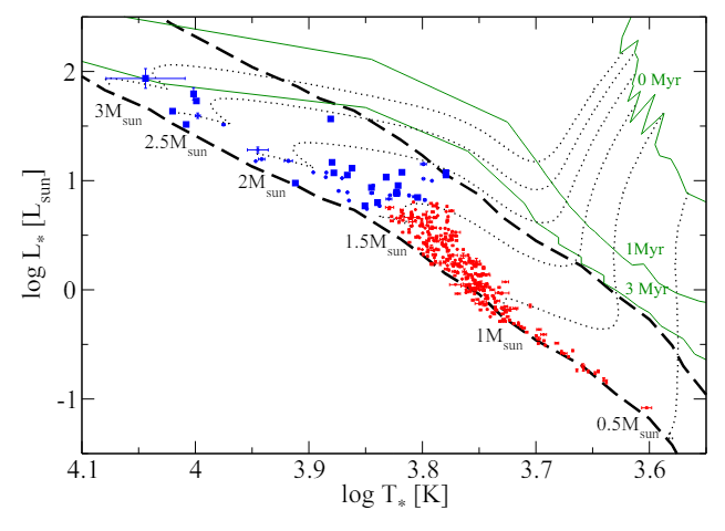
\ Figure B.1 shows the Hertzsprung-Russell (HR) diagram of the TOIs, adding to the intermediate-mass sample the 298 lowmass stars. All these host planets with CP and KP classification status (Appendix A) and are plotted in red. Planets without such a classification around intermediate-mass stars (22 out of 47) are represented with blue squares. We also plotted the lower and upper dashed lines representing the beginning and the end of the MS phase (for details about the MS evolution, see, e.g., Salaris & Cassisi 2006). In addition, pre-MS tracks and isochrones from Siess et al. (2000) are indicated for a representative set of stellar masses and ages (see Appendix C).
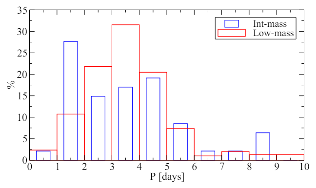
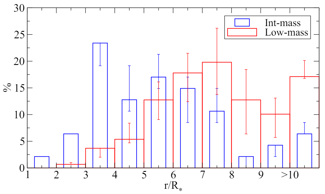
\ With respect to the properties of the planets, Fig. B.2 shows the planetary radii and orbital periods for the TOIs in the sample. Planets around intermediate-and low-mass stars, as well as their classification status, are again indicated. Planet sizes in between that of Neptune and a few Jupiter radii homogeneously distribute along the whole range of periods for the intermediate and low-mass samples. Figure B.3 compares the distribution of orbital periods around intermediate- and low-mass stars. Planets around intermediate-mass stars peak at 1-2 days, contrasting with the “three-day pileup” of the population of hot Jupiters around low-mass stars observed here and, in the literature, (e.g., Yee & Winn 2023, and references therein). Apart from this, the distributions of periods are similar for both stellar mass regimes. Indeed, a two-sample K-S test does not reject the null hypothesis
\ 
\ 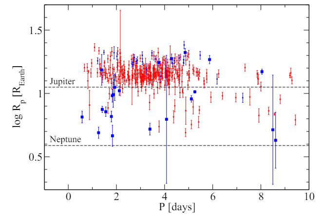
\ that the orbital periods around intermediate- and low-mass stars are drawn from the same parent distribution, at a significance level given by p-value = 0.0957.
\ The similarity between the distributions of TESS planet sizes and periods explored in this work (Figs. B.2 and B.3) suggests that the intermediate- and low-mass stars samples are similarly affected by potential observational biases. Thus, such biases should not originate the differences between both samples reported here (see Sect. 3).
\ 
\ 
\ 
\
Appendix C: Pre-MS estimates
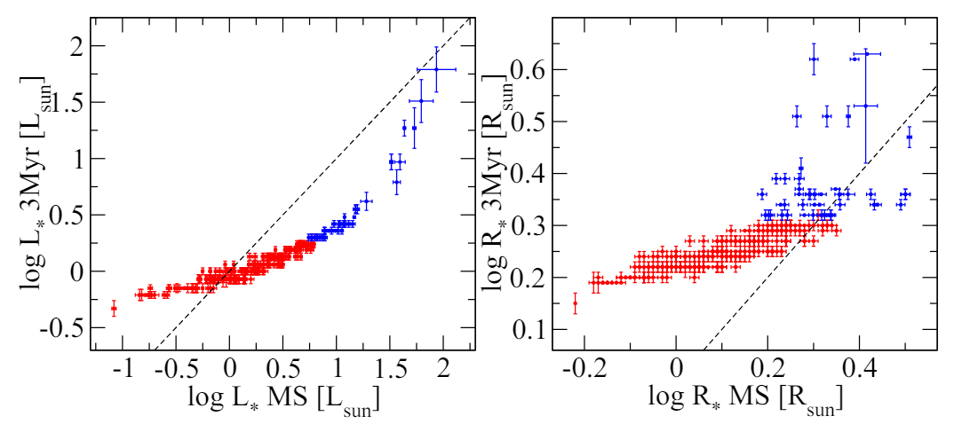
The Siess et al. (2000) isochrones provide, for a given age and metallicity, the corresponding values of the stellar parameters L∗, R∗, T∗, and M∗. In turn, the pre-MS evolution in the HR diagram can be inferred, for a given value of M∗ and metallicity, from the Siess et al. (2000) evolutionary tracks. Based on the Gaia DR3 stellar masses, the pre-MS values of L∗ and R∗ were inferred for each star in our sample using the 3 Myr isochrone from Siess et al. (2000), assuming solar metallicity. This isochrone is plotted in Fig. B.1, along with several representative evolutionary tracks. From this graphical perspective, the pre-MS values for a given stellar mass are inferred from the point where the 3 Myr isochrone and the corresponding evolutionary track coincide. Figure C.1 compares the MS luminosities and radii from Gaia DR3 with those estimated during the pre-MS at 3 Myr. Errorbars in the y-axes reflect the uncertainties in the Gaia DR3 stellar masses used to infer the pre-MS values of L∗ and R∗ based on the isochrone, and also take into account the fact that bins of 0.1M⊙ were assumed to be interpolated.
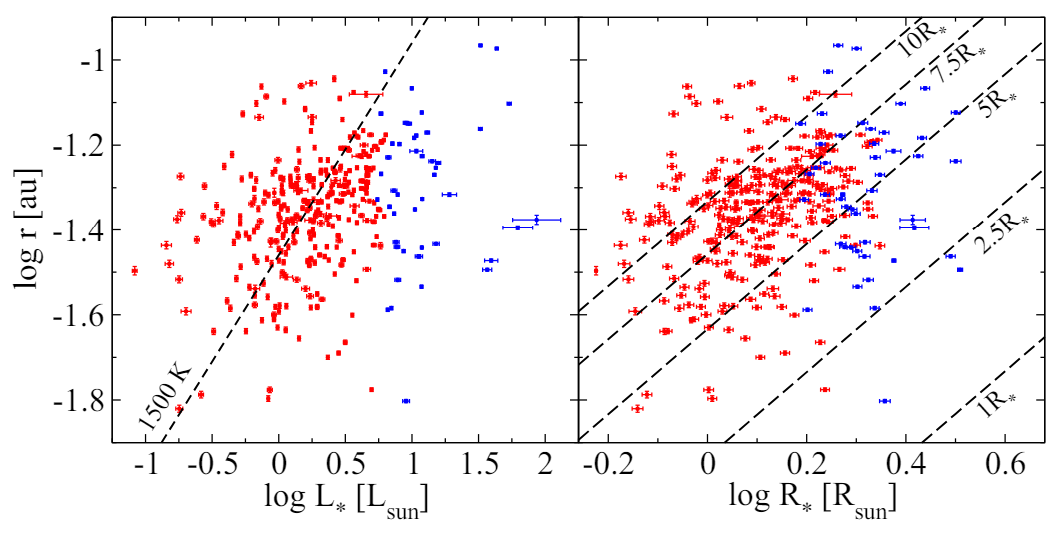
\ To estimate how disk dissipation timescales different than the typical 3 Myr affect our results and conclusions, we considered two cases. First, it was assumed that disk dissipation in intermediate-mass stars is faster than in low-mass stars. This difference has been suggested in earlier works indicating that disks around intermediate- and low-mass stars dissipate mostly at ∼ 1 Myr and ∼ 3 Myr, respectively (e.g., Ribas et al. 2015). The 1 Myr isochorne from Siess et al. (2000) is plotted in Figure B.1 along with the 3 Myr isochrone. For a typical intermediate-mass star with M∗ = 2M⊙, L∗ at 1 Myr is ∼ 0.2 dex larger than at 3 Myr. Because T∗ is slightly smaller at 1 Myr, R∗ at this age is larger by a factor ∼ 1.4 (0.1 dex) compared with that at 3 Myr. The net result is a slight displacement of the intermediate-mass stars to the right of both panels in Fig. 2, and to the left in Fig. 3. In other words, our conclusion that planetary orbits around intermediate-mass stars tend to be smaller than the dust-destruction radius and consistent with small magnetospheres would be reinforced under this scenario.
\ 
\ 
\ 
\ In addition, compared with the previously discussed changes of the disk dissipation timescale, the use of metallicities that are different than solar or evolutionary tracks and isochrones different to those in Siess et al. (2000) have a negligible effect on the pre-MS values inferred for L∗ and R∗ (see, e.g., Siess et al. 2000; Stassun et al. 2014).
\ In summary, although different assumptions to infer the stellar luminosities and radii during disk dissipation have an effect on their specific values and related statistics, the general results and conclusions of this work remain unaltered.
:::info Authors:
(1) I. Mendigutía, Centro de Astrobiología (CAB), CSIC-INTA, Camino Bajo del Castillo s/n, 28692, Villanueva de la Cañada, Madrid, Spain;
(2) J. Lillo-Box, Centro de Astrobiología (CAB), CSIC-INTA, Camino Bajo del Castillo s/n, 28692, Villanueva de la Cañada, Madrid, Spain;
(3) M. Vioque, European Southern Observatory, Karl-Schwarzschild-Strasse 2, D-85748 Garching bei München, Germany and Joint ALMA Observatory, Alonso de Córdova 3107, Vitacura, Santiago 763-0355, Chile;
(4) J. Maldonado, INAF – Osservatorio Astronomico di Palermo, Piazza del Parlamento 1, I-90134 Palermo, Italy;
(8) B. Montesinos, Centro de Astrobiología (CAB), CSIC-INTA, Camino Bajo del Castillo s/n, 28692, Villanueva de la Cañada, Madrid, Spain;
(6) N. Huélamo, Centro de Astrobiología (CAB), CSIC-INTA, Camino Bajo del Castillo s/n, 28692, Villanueva de la Cañada, Madrid, Spain;
(7) J. Wang, Departamento de Física Teórica, Módulo 15, Facultad de Ciencias, Universidad Autónoma de Madrid, 28049 Madrid, Spain.
:::
:::info This paper is available on arxiv under CC BY-SA 4.0 DEED license.
:::
[2] https://tev.mit.edu/data/
\ .[3] https://exoplanet.eu/home/
Ayrıca Şunları da Beğenebilirsiniz

Trump Cancels Tech, AI Trade Negotiations With The UK
Egrag Crypto: XRP Could be Around $6 or $7 by Mid-November Based on this Analysis